Uncertainty Measurement Analysis
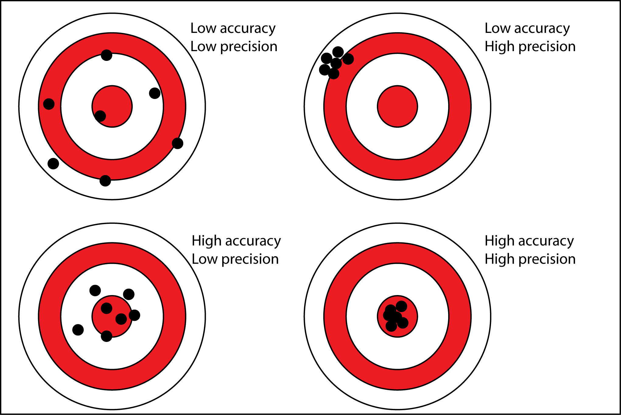
Experience shows that all measurements are subject to uncertainty, since none can be exact, and understanding the level of uncertainty tells us how reliable a measurement is. Measuring tools likewise can never be 100% correct. Thus, the accuracy of our engineering measurements indicate how close our measurements are to the true value. Yet, sometimes the true value cannot be quantified since it might be difficult to measure it. For example, there is a high possibility that during our ultrasonic distance measurements we placed the block not exactly on the inch mark of the ruler. By not being able to know exactly the true value of the measurements, engineers use the repeatability of the measurements to describe their precision. The game of throwing darts on a target illustrates very well the difference of accuracy and precision. Generally, a low accuracy but high precision situation indicates a potential systematic error as opposed to random errors when we get low accuracy and low precision. As we can see, the concept of precision is related to the level of variance in the data. The smaller the variance the higher the precision.
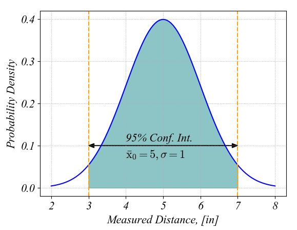
Because we just estimate the true value and we only know the measured values, we do not know the exact values of errors. Thus, we estimate the range of probable errors based on what we know about our measurements. This estimation is called the uncertainty of the measurements. For this we need to calculate the mean values and the standard deviations at each measurement location. We will also quantify the confidence interval about the measured mean value at each location for the given 95% probability specific to engineering field. This confidence interval is the interval around the mean value containing 95 data points from 100 measurements that we would take. For example, the following figure illustrates the normal distribution for a set of measurements having the mean value of x̄ 0 = 5 and a standard deviation σ = 1. Statistically, the 95% confidence interval ranges from x̄ 0 - 2σ to x̄ 0 + 2σ. You can find the python code to plot this normal distribution and confident interval in this pdf file.
The following video shows how we can import the raw data from the previously saved file and explains the Python program that sorts through the data file, calculates averages and confidence intervals, and plots this processed data with errorbars. The explanations of my Python file that I use in this tutorial video are found in this pdf file.
Data Analysis in Python
The following Python script (discussed in the previous video, above) shows how we can extract the measurement values at each location along the ruler, then how we can calculate the mean, standard deviation, and confidence intervals. First, the code imports the comma separated data file that you saved during the previous assignment. At the end of all calculations, the results are graphed in a figure indicating the mean and the confidence intervals with error bars. To run this script, please copy it and paste it in your python editor.
#-------------------- Rational of the data analysis code ---------------------------
# This code does the follwing:
#     1) extracts the distance values from the csv data file (that we measured
#        previously)
#     2) sorts these values for each position where we measured
#         *  I measured mine in a range of 1 to 20-inch in increments of 1-inch
#     3) Calculates the mean value and the stardand deviation from the sorted
#        values of each location
#     4) Plots the mean values with error bars at 95% Confidence Intervals
#     5) Compares these mean values with the true values that we expected to have,
#        i.e. 1, 2, 3, ... 20-inch

# --------------- Import modules that we need --------------------------------------
import numpy as np
import matplotlib.pyplot as plt


# Some additional commands (at your choice) to set font globally
# as times new roman, italic, and bold for nicer plots
plt.rcParams["font.family"] = "Times New Roman"
plt.rcParams["font.style"] = 'italic'
plt.rcParams["font.weight"] = 'bold'
plt.rcParams["font.size"] = 14

# -------------------- Import the csv data file that was saved --------------------
dat = np.loadtxt('Distance_Measurement_Wood_block.csv', delimiter=',', skiprows = 1)
Time = dat[:,0] # The first column was time in seconds
Dist = dat[:,1] # The second column was the distance


Means = []# Create an empty array of to collect the mean values as they are extracted
Stds = [] # Create an empty array of the standard deviation values

# --------- Separate Distance Data in Bins of 1, 2, 3, ... 20-inch (in my case) -----
# Use a for loop to collect all the distance values that fall within a range of
# -0.5 inch to +0.5 inch of the intended distance.
#       For example, all the measured distance values between 0.5 to 1.5-inch will be
#       collected in the bin for 1-inch distance

for i in range(1,21):
    # the 'where' numpy function helps to get the indexes of the values
    Indexes = np.where(np.logical_and(Dist >= i-0.5, Dist <= i+0.5))
    Sorted = Dist[Indexes]# Drop the distance values within each bin
    Mean = np.mean(Sorted)# Calculate the mean value of the bin
    Std = np.std(Sorted)  # Calculate the standard deviation value of the bin
    Means.append(Mean)    # Append the calculated mean value in the array
    Stds.append(Std)      # Append the calculated std in the array

# ---- In case that we want to see how the analysis works until this point
print("mean = ",Means)
print('Std = ',Stds)

# Generate an array of equally spaced values from 1 to 20 as our true values
TrueValues = np.linspace(1,20,20)

# Calculate the Confidence Intervals as two standard deviation above and two standard
# deviation below the mean value. This is required to get a probability of 95%
CI = np.multiply(Stds,2)

Mean_CI = np.nanmean(CI) # Calculate the mean value, any nan, "not a number", is removed
print('Mean CI: ',Mean_CI)

# ------------- Plot the Measured Distance and Its Confidence Intervals ------------
fig = plt.figure(1)
plt.clf()
plt.errorbar(TrueValues,Means,yerr=CI,fmt ='bo', markerfacecolor='none',
             capsize=2,ecolor='red', label='Measured')

plt.plot(TrueValues,TrueValues,'--b.', label='Expected Value')
plt.xlabel('Distance, true value, [in]')

plt.ylabel('Measured distance, [in]')
##plt.axis([0, 5, -3, 4])
plt.grid(True)
plt.grid(linestyle='dotted')
ax = plt.gca()
ax.set_position([0.15,0.17, 0.75, 0.75])# adjust margins of the figure
plt.legend()# show legend on the graph


plt.show()# needed when we use IDLE
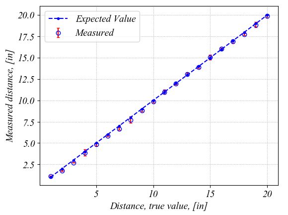
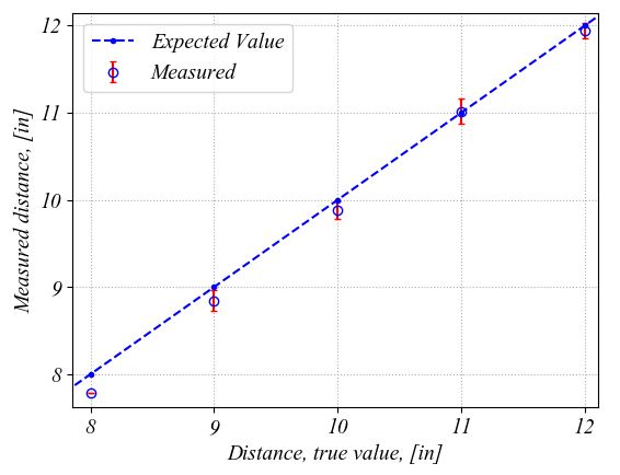
Python plots the following figure. The plot on the right is a zoom in to better show the errorbars and the markers. The errorbars represent the 95% confidence intervals with two stardard deviations above and below the mean value for each location. As we talked above, the true value on the graph represents an estimated value. It is here just for a comparison with the distance measured with the ultrasonic transducer. These plots show that overall, the ultrasonic transducer performs well. In some locations, the errorbars are larger and this might be caused by the fact that I might have move the wood block slower and I captured points while I was moving it.
|
|
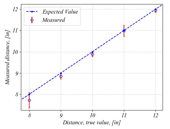
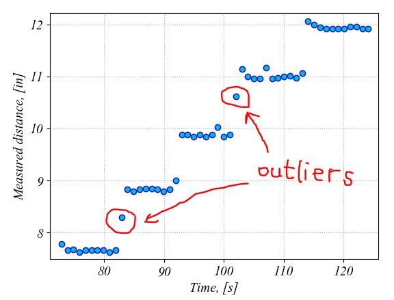
If we change the indexes search range in the for loop, i.e. the "Indexes" line in the for loop, from ± 0.5 from the expected value to ± 0.25, then the precision is increased. This means that the 95% confidence intervals are much tighter this time as it can be seen in the following zoom in the figure. By using a tighter range for selection of the measured distance values at each location, we remove the outliers that were introduced from moving the wood block too slow in the desired position. For example, such outliers were removed from locations at 8-inch and 11-inch distance from the transducer by using a tighter selection interval when calculating the mean and standard deviation values.
|
|
Thus the smaller the confidence intervals are the higher the precision of the measurement will be. After we removed the outlier data points caused by recording data while moving the block into the position, the 95% confidence interval has an average value of ± 0.11-inch. We use the average value to characterize the confidence intervals since we want to minimize the effect of other features of our measurement setup. The average value is an indication of the precision of the whole measurement setup, not only of the ultrasonic transducer. As we have seen in the previous assignment, a tilt of the block might introduce errors in our measurements. Moreover, any loose jumper wire can also affect the precision. Thus, the final conclusion is that with our current setup, 95 points out of 100 fall within ± 0.11-inch of the mean value that represents the measured distance.